Lab: Hard Disk Drives

CSC 213 - Operating Systems and Parallel Algorithms - Weinman

Summary:

You will experiment with I/O timing for a simulated hard disk drive.

Objectives:

Practice computing seek, rotation, and transfer times for requests
Understand the impact of seek rate, rotational delay, and scheduling algorithm on I/O times

Exercises

Preliminaries

Do this laboratory on any MathLAN workstation. You don't need to copy any starter files, simply change your working directory as follows.

: $ cd ~weinman/public_html/courses/CSC213/2012F/labs/code/disk

Part A: Basics

Compute the seek, rotation, and transfer times for the following requests. The -G option launches the graphical interface, but you should read the disk details from the terminal to do your calculations before starting the simulator.

./disk.py -G -a 6
./disk.py -G -a 30
./disk.py -G -a 7,30,8
Repeat the last request above, but using different seek rates.
1. Use a seek rate of 10 distance units per time unit:
  
  ./disk.py -G -a 7,30,8 -S 10
2. Use a seek rate of 0.1 distance units per time unit:
  
  ./disk.py -G -a 7,30,8 -S 0.1
How do the times change?

Part B: Scheduling

You may have noticed that some requests streams would be better served with a policy other than FIFO.

For the request stream 7, 30, 8, what order should the requests be processed in?
Using the shortest seek-time first (SSTF) disk scheduler what should the seek, rotation, and transfer times be?
Verify your answer:

./disk.py -G -a 7,30,8 -p SSTF
Using the shortest access-time first (SATF) scheulder, what order should these requests be serviced in?
Find a set of rquests where SATF does noticeably better than STF; what are the conditions for a noticeable difference to arise? (Be prepared to discuss your answer with the class.)

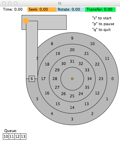
Part C: Geometry

Try the request stream 10, 11, 12, 13 with FIFO and the default parameters:

./disk.py -G -a 10,11,12,13
This request is not handled particularly well. Why?
The simulator includes a track skew option, measured in blocks. For example, the simulation on the left shows the default skew of zero, while the simulation on the right shows the a skew of one.

Track skew = 0 Track skew = 1

Given the default seek rate, what should the skew be to minimize the total time for this request? Why?
Verify your answer:

./disk.py -G -a 10,11,12,13 -o skew

If you were wrong, revise your explanation, not just your number.
What should the skew be if the seek rate is four distance units per time unit?

For those with Extra Time

You may choose any one (or more) of the following exercises that interest you.

Extra 1: Dense outer tracks

Multi-zone disks pack more blocks into the outer tracks. To configure this disk in such a way, run with the -z flag.

Specifically, try running some requests against a disk run with -z 10,20,30 (the numbers specify the angular space occupied by a block, per track; in this example the outer track will be packed with a block every 10 degrees, the middle track every 20 degrees, and the inner track with a block every 30 degrees).
Run some random requests (e.g., -a -1 -A 5,-1,0, which specifies that random requests should be used via the -a -1 flag and that five requests ranging from 0 to the max be gneerated), and see whether you can compute the seek, rotation, and transfer times. Use different random seeds (-s 1, -s 2, etc.).
What is the bandwidth (in blocks per unit time) on the outer, middle, and inner tracks?

Extra 2: Scheduling windows

Scheduling windows determine how many block requests a disk can examine at once in order to determine which block to serve next.

Generate some random workloads of a lot of requests (e.g., -A 1000,-1,0, with different seeds, perhaps) and see how long the SATF scheduler takes when the scheduling window is changed form 1 up to the number of requests (e.g., -w 1 up to -w 1000, and some values in between).
How big of scheduling window is needed to approach the best possible performance?
Note: Use the -c flag and don't turn on the graphics with -G to run these more quickly.
When the scheduling window is set to 1, does it matter which policy you are using?

Extra 3: Starvation

Avoiding starvation is important in a scheduler.

Can you think of a series of requests such that a particular block is delayed for a very long time given a policy such as SATF?
Given that sequence, how does it perform if you use a bounded SATF (BSATF) scheduling approach? In this approach, you specify the scheduling window (e.g., -w 4, see prior problem above) as well as the BSATF policy (-p BSATF); the scheduler will then only move on to the next window of request when all of the requests in the curent window have been serviced.
Does this solve the starvation problem? How does it perform, as compared to SATF?
In general, how should a disk make this trade-off between performance and starvation avoidance?

Extra 4: Greedy vs. Optimal

All the scheduling policies we havce looked at thus far are greedy, in that they simply pick the next best option instead of looking for the schedule over a set of requests. Can you find a set of requests in which this greedy approach is not optimal?

Acknowledgment:: Exercises and disk.py from Operating Systems: Three Easy Pieces ("Hard Disk Drives") by Remzi H. and Andrea C. Arpaci-Dusseau.

Track skew = 0	Track skew = 1