Lab: Structure from Motion
CSC 262 - Computer Vision - Weinman
- Summary:
- You will use a given set of very dense feature matches to create a 3-D orthographic reconstruction.
Deliverables
- The Matlab script used to make your comparisons and generate your report
- (5 points) Top singular values from decomposition (B.3)
- (10 points) Image of 3-D shape of reconstruction (C.1)
- (10 points) Observations of reconstruction (C.2)
- (10 points) Synthesized 3-D views of scene (D.5)
- (10 points) Commentary on synthesized views (D.6)
- (25 points) 3-D views of sparse/noisy reconstruction (E.4) As generated by the following processes (commented within the script, but not displayed in the report)
- (10 points) Observations of sparse/noisy reconstruction (E. 5)
- (10 points) Professionalism of write-up
Preparation
Load one of the following synthetic images that you'd like to build a 3-D reconstruction of.- /home/weinman/courses/CSC262/images/frame1.png /home/weinman/courses/CSC262/images/gframe1.png
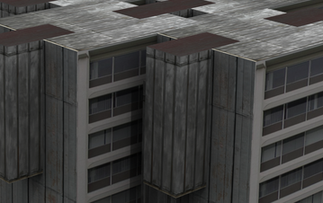 | 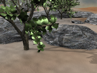 |
| frame1.png | gframe1.png |
- >> load /home/weinman/courses/CSC262/images/flow.mat % For frame1.png >> load /home/weinman/courses/CSC262/images/gflow.mat % For gframe1.png
Exercises
A. Set Up
- Use meshgrid to construct the 2-D spatial domain (x and y coordinates in two matrices) of the pixels in frame1. Note: Remember that the first dimension of a matrix is the rows, and the second dimension is the columns, which is the reverse of the typical (x,y) pair ordering.
-
Now that you have matrices representing (x,y)
pairs of points in the image, use the data in the variable F
to create matrices of the coordinates of their corresponding points
in frame2. That is, if X1(a,b) and Y1(a,b)
are the x and y coordinates of a point (a,b) in frame1,
then you should create matrices X2 and Y2 such that
X2(a,b) and Y2(a,b) are the coordinates of the same
(real) point in frame2 using the relations
x2 = x1+Fx y2 = y1+Fy - Construct a complete 4×N data matrix of the two frames' points. That is, the x coordinates from the first image should be the first row, the x coordinates of the matching points from the second image should be the second row, and similarly with the y coordinates for the third and fourth row.
- Calculate the translation of the points perpendicular to the viewing direction (i.e., find the mean of each row).
- Create a modified data matrix where the row mean (centroid) has been subtracted from each value in the data matrix.
B. Factorization
-
You should now have a matrix suitable
for singular value decomposition (SVD). Using the Matlab command,
decompose the data matrix into its constituent factors, i.e.,
- [U,W,V] = svd(X,'econ');
- Extract W3, the 3×3 sub-matrix of W containing the top three singular values and V3, the corresponding columns from V (an N×3 matrix).
- What are the three singular values you find? What do they tell you?
- Take the product of the two extracted matrices from B.2 in order to recover the shape matrix S*.
C. Analysis
- The first and second rows of your shape matrix S* contain the
(arbitrary) X and Y coordinates of the recovered 3-D points.
In order to construct a full 3-D plot of these points in a connected
fashion, we will use what is called a Delaunay triangulation. This
connects the recovered points with triangles. Use the delaunay
Matlab command to create a plot structure from your points, i.e.,
- T = delaunay(X,Y);
-
Next we plot a simple visualization of the
3-D structure recovered by algorithm. The command trisurf
takes a set of x, y, and z coordinates and plots them using
the Delaunay triangles we created in the previous step. Use the coordinates
from your shape matrix to render the recovered scene structure. One
suggested syntax is
- trisurf(T, X, Y, Z, 'EdgeColor', 'none', 'FaceColor','red'); lighting phong
- view([-161 46]);
- [camAzim,camElev] = view();
- camlight headlight
- Use the 'Rotation 3D" tool in the figure window to adjust the view and inspect the structure. After you find an interesting view (the azimuth and elevation are reported for you within the figure window), programmatically set the figure to use this view (i.e., in your published report) with the view command. Note: you should do this secondary view change after installing the light with camlight).
- Does the structure look like you expect? Are there any 3-D structures that appear that you did not necessarily expect?
D. Visualization
Visualizing the surface by shape alone is helpful, especially for finding flaws, but is unsatisfying visually. Fortunately, Matlab allows the surface faces to be colored by an index.- If you haven't already, load an RGB version of frame1.png.
- Use the command rgb2ind to convert the image to an indexed image using 256 colors. You will need to specify both the indexed image and the colormap as outputs.
- Reshape the resulting imaged index into a column vector.
-
Now you can use the resulting index vector
as an additional argument to trisurf, which will indicate
the color to use in the rendering. For example,
- figure; trisurf(T, X, Y, Z, C, 'EdgeColor', 'none'); colormap(map);
- Use the "Rotation 3D" tool to synthesize at least two novel views of the scene using view and snapnow.
- What do your views help to illustrate about the 3-D structure?
E. Reality
Usually, matching is more unreliable and much sparser than the data we have used so far. In this section you'll explore a simulated, but more realistic reconstruction scenario.- Return to just "between" A.5 and B.1 and reduce the number of matching coordinate points you use in your factorization. You should try devise a way to sample them non-uniformly. Hint: use randi to get integer indices (i.e., for the data matrix columns).
- Using your much smaller set of points add some random noise to the offsets; that is, the matching points (originally calculated in A.2) should be additively disturbed. Hint: Use randn, which produces number from the "standard" normal distribution (zero mean, unit standard deviation). Even small errors multiply greatly for points at large distances. You may wish to investigate the magnitudes of the typical match offsets before choosing a multiple to alter the standard deviation of the noise.
- Carry out the remainder of the steps for doing orthographic structure from motion on your reduced, noisy data.
- Display two visualizations of your data: one that is a solidly colored shape (as in C.2) and another that is color-mapped (as in D.4). You will likely need to experiment with the amount of sparsity and noise you inject before getting a vaguely satisfying result.
- Comment on the quality of the reconstruction. Based on your explorations, which issue (noise or sparsity) may have bigger impact on the quality of the result? Justify your claim.
Acknowledgments
The images and flow ground truth are from the Middlebury Optical Flow data set (Synthetic Grove2 and Urban2 images), which proclaims:If you report performance results on our benchmark, we request that you citeA Database and Evaluation Methodology for Optical Flow, published open access in International Journal of Computer Vision, 92(1):1-31, March 2011.
Copyright © 2010, 2012, 2015, 2019, 2020, 2022 Jerod
Weinman.

This work is licensed under a Creative
Commons Attribution-Noncommercial-Share Alike 4.0 International License.