Figure 1. As in this 1896 bicycle trail map of California's central valley, historical maps feature irregular typefaces, overlapping text and graphical elements, and text with curved baselines and arbitrary orientation. detail. (Credit: Image 1592006 © Cartography Associates

Maps tell tales of politics, people, and progress. Historical and print map collections are important library and museum holdings frequently available only to scholars with physical access. Fortunately, many are now being digitized for more widespread access via the web.

Unfortunately, most maps are only coarsely indexed with meta-data, increasingly even georectified, while the contents themselves remain largely unsearchable. The goal of this project is to further increase the accessibility of information locked in geographical archives by automatically recognizing place names (toponyms).

Figure 2. Graphical probability model (Bayesian network) for toponym recognition. Greyed ovals are observed values, and values inside the plate are replicated N times, once for each word to be recognized in the map. (Copyright © 2017 IEEE. Used by permission.)

For a set of word images from the map and their and image coordinates, we seek the strings, projection, and alignment that maximize the joint probability described by the Bayesian model at right (Figure 2). To support this, the model associates the underlying category and specific feature represented by each word with the typographical style in which it is rendered.

The global georectification alignment relates image coordinates to a gazetteer of known feature locations projected into the same Cartesian plane. We search for an initial maximum likelihood alignment with RANSAC and refine the result with Expectation Maximization.

Figure 3. Learning process for the Bayesian model. Outputs are cumulative and displayed only where updated. (Copyright © 2017 IEEE. Used by permission.)

A general robust word recognition system (a deep convolutional network with a flexible parser) produces a ranked list of strings and associated prior probabilities. We then use the most probable cartographic projection and alignment to update posterior probabilities for the recognized strings.

Taking the initial alignment from multiple cartographic projection families as a starting point, we refine the model parameters by expectation maximization. Later stages consider entities from additional geographic categories with appropriate cartographic models, allowing label words to be positioned anywhere along river flowlines or within regional boundaries (more below).

Finally, using an a priori clustering of words into text styles, we correlate style and geographic categories to finalize the bias among geographic features and rerank recognitions with Bayesian posteriors.

To detect words in maps, we have created the MapTD network, an adaptation of EAST (Zhou et al., 2016). The structure of the network is shown below.

Figure 4. Map Text Detector (MapTD) network structure. ResNet-50 performs feature extraction (top row) for an input image. Feature merging (middle row) upsamples and concatenates outputs from neighboring layers, providing a final feature map for the output layers (bottom row). (Copyright © 2019 IEEE. Used by permission.)

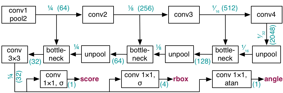
One key difference between MapTD is trained to predict the semantic orientation of a word rectangles, whereas EAST is trained to predict the geometric orientation. This change boosts end-to-end detection and recognition performance by 3.6%.

There are several other smaller differences. First, rather than directly regress the distances using the raw convolutional outputs, MapTD uses a sigmoid to compress values to the range (0,1) for stability. To reconstruct boxes, these compressed results are multiplied by the training image size. Second, MapTD uses Dice loss to train the detection scores, rather than the class-balanced cross-entropy used by EAST.

Example detection results trained using ten-fold cross-validation on the annotated dataset of 30 maps appear in Table 1 below, with an example in Figure 5.

Figure 5. Detected text rectangles (predicted baseline in blue). (Copyright © 2019 IEEE. Used by permission.)

Figure 6. Relevant probabilities for the word "Pensacola". Left: Given the alignment, the predicted location of the best toponym (2404503: City of Pensacola) is shown at the mean of the likelihood, surrounded by three isotropic standard deviations. Right: prior and posterior probabilities for top candidate strings. (Copyright © 2013 IEEE. Used by permission.)

In these results, geographical information enables us to infer coarse georeferencing of historical map images from noisy OCR output. The table at right lists error percentages and harmonic mean of correct words' ranks using twenty maps with 6,949 words where the correct string was ranked by the original OCR and present in the gazetteer. Jointly inferring toponym hypotheses and gazetteer alignment eliminates 37% of OCR errors.

Figure 7. Corresponding state shape outline as a RANSAC search progresses to higher-scoring alignments. (Credit: Map Image 1070001 © Cartography Associates)

The animation at left shows alignments as the RANSAC-based search progresses to higher scores, a process which takes about 20 seconds after fewer than 500 random samples. Note that only the extracted words and their locations are used to determine the alignment no other image information, such as boundary contours. Reranking OCR scores using the final alignment reduces word recognition error in this image from 44% to 24%.

The figure below shows word recognitions and their posterior probabilities overlaid on a region of a map with complex artifacts. One recognition is marked incorrect and has a lower a score because the 1860's era map uses an unconventional spelling, and the spatial alignment pushes the system to produce its modern name.

Figure 8. Overlaid posterior word recognitions and scores. (Credit: Map Image 1070006 © Cartography Associates)

Style and Category Modeling

Maps may pictorially and textually represent entities from a wide variety of categories, from cities to rivers or administrative regions. To support these additional categories as well as the tendency of a map, atlas, or geographic region to exhibit bias among them, we automatically link the category to a learned typographical representation of the text labels' styles.

The figure below demonstrates how the model clusters words by style according to their category, representing primarily water features (italics), city names (standard font), and counties or states (all capital letters).

Figure 9. Text style clusters. Word images are ranked by probability of containing an LDA-based [Blei03] style (k=4) using LBP features [Nicolau15]. (Credit: Map Image 5242001 © Cartography Associates)

Figure 10. Comparison of example ground truth and learned style-conditional category probabilities from two of the clusters above.

The figure at right illustrates how the style clusters can induce appropriate bias for particular geographical categories. Without any style information, the geographical entities for the map are determined to be mostly city or town placenames or counties (by a 2:1 margin), with a few rivers, lakes, and other outliers. We can see the uncertainty drastically reduced among several style clusters, which here separate placenames and counties into individual clusters, giving them an appropriate bias.

Non-point Feature Labels

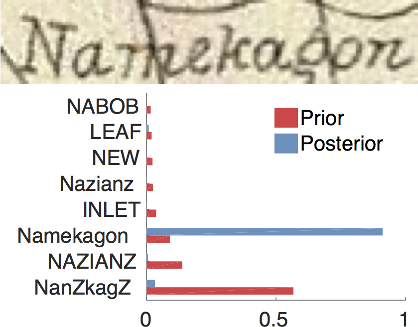
Given a georeferenced map, predicting the location of a label for a small-scale point feature may be done with straightforward Gaussian model, which efficiently penalizes the squared distance betweeen the geographic prediction and the cartographic representation (see Figure 6). Because rivers and large lakes or counties do not fit this formulation, we instead penalize the minimum distance between the cartographic representtation and the geographic prediction, which is now a polyline or polygon. Binarizing the known shape on the image grid allows us to use a linear-time distance transform algorithm for effiency. The figure below shows an example of likelihood function, predicting where a label should appear for a particular geographic feature in a georeferenced map, along with the corresponding prior (OCR alone) and posterior (OCR plus georeferenced likelihood) probability distributions.

Figure 11. River name recognition: contours of polyline likelihood (1579990: Namekagon River) and comparison of prior (using OCR alone) and posterior (adding automatic georeferencing) probability distributions. (Copyright © 2017 IEEE. Used by permission.)

Part of the success of the recognition process depends on having sufficient training data. Because annotated data is limited, we synthesize map text. It is important that such synthetic data be realistic. Rather than generate a static dataset, which could allow a highly parameterized deep network to overfit, we create a dynamic pipeline that quickly renders synthetic text on-the-fly for training. In this way, the model never sees the same example twice during training and must therefore learn the general patterns in the data, rather than memorizing specific images.

Figure 12. Dynamic map text synthesis. Top: Synthesis pipeline. Middle: Example images. Bottom: Real word images cropped from maps. (Copyright © 2019 IEEE. Used by permission.) clusters above.

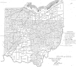
Aligning map images with geographical coordinates is a painstaking, time-consuming manual process. The text-only approach detailed above is susceptible to systematic errors. To improve on those results, this work aligns historic maps to a modern geographic coordinate system using probabilistic shape-matching.

Starting from the approximate initial alignment given by the toponym recognition, we then optimize the match between a deformable model built from GIS contours and ink from the binarized map image. On an evaluation set of 20 historical maps from states and regions of the U.S., the method reduces average alignment RMSE by 12%.

Original	Binarized Ink	Model	Final Fit

Figure 13. Example inputs (left) and final result of alignment process. (Copyright © 2019 ACM. Used by permission. Credit: Map Image 1070001 © Cartography Associates)

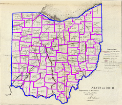
The model deforms control points of a GIS shape to better match ink locations, while retaining a bias for the original shape. Generally, models seek part locations that minimize the squared minimum distances to image ink and deviations from expected model part positions. Dense correspondences arise from a parametric affine fit or a robust thin plate spline (TPS).

Minimization is exact for acyclic, tree-shaped models. However, most GIS models are represented as cyclic graphs. To compensate, we embed model part locations within belief functions. Iterative belief updates subsequently penalize both the part's distance from image ink and deviation from the preferred model shape while considering neighbor’s part location beliefs.

Figure 14. Left: Initial fit from toponym-based alignment. Right: Final fit from deformable model and robust thin-plate splines. (Copyright © 2019 ACM. Used by permission. Credit: Map Image 1070005 © Cartography Associates)

• Deformable Part Models for Automatically Georeferencing Historical Map Images In ACM International Conference on Advances in Geographic Information Systems (SIGSPATIAL), Nov. 2019. 🏆 Best Poster Award. [paper] [poster] [bib] [doi] [tech report]
• Deep Neural Networks for Text Detection and Recognition in Historical Maps. In International Conference on Document Analysis and Recognition (ICDAR), September 2019. [PDF] [bib]
• Geographic and Style Models for Historical Map Alignment and Toponym Recognition. In International Conference on Document Analysis and Recognition (ICDAR), November 2017. [PDF] [bib] 🏆 Best Paper Award
• Toward Integrated Scene Text Reading. IEEE Transactions on Pattern Analysis and Machine Intelligence (PAMI), 36, Feb. 2014. [PDF] [bib]
• Toponym Recognition in Historical Maps by Gazetteer Alignment. In International Conference on Document Analysis and Recognition (ICDAR), August 2013. [PDF] [bib]

• Sources (31 MrSid files; 131M; MD5) [DOI:11084/10473]
• Images (31 TIFF files; 1782M; MD5) [DOI:11084/19499]

We gratefully acknowledge the David Rumsey Map Collection as the source of the map images, which come with the following notice:

Images copyright © 2000 by Cartography Associates. Images may be reproduced or transmitted, but not for commercial use. ... This work is licensed under a Creative Commons [Attribution-NonCommercial-ShareAlike 3.0 Unported] license. By downloading any images from this site, you agree to the terms of that license.

Complete Annotations

These annotations are used in the ICDAR 2019 paper and mark all the words and characters in the map images.

• Annotations (31 JSON files) [DOI:11084/23296]
• Brief Description (PDF) [DOI:11084/23295]

An archived version of this data set is permanently available at http://hdl.handle.net/11084/23294

Georeferencing Correspondences

These corresponding image and geographical coordinate points are used in the SIGSPATIAL 2019 paper.

• Correspondences (33 TXT files) [DOI:11084/23332]
• Brief Description (PDF) [DOI:11084/23331]

An archived version of this data set is permanently available at http://hdl.handle.net/11084/23330

Toponym Annotations

These annotations are used in the ICDAR 2017 paper and are designed for toponym recognition, rather than text/graphics separation because several non-toponym words are not marked.

• Annotations (31 XML files; 1.1M) [DOI:11084/19494]
• Annotations+GNIS ID (7 XML files; 179K) [DOI:11084/19495]
• Gazetteer Regions (31 TXT files; 1.6K) [DOI:11084/19496]
• Brief Description (PDF) [DOI:11084/19493]

An archived version of this data set is permanently available at http://hdl.handle.net/11084/19349

The 12 map annotations used in the 2013 ICDAR paper are available at http://hdl.handle.net/11084/3246

Ground Truth Processing Code

The following Java code processes and stores data from these XML annotations. The Matlab code uses the Java objects to produce cropped, normalized word images.

• map.tar (Java and Matlab source) [DOI:11084/19498]
• map.m (README Matlab source) [DOI:11084/19497]

This repository contains our Tensorflow implementation of MapTD from Weinman et al. (2019), described above.

• github:weinman/MapTD [DOI:11084/23321]
• Model checkpoints from paper (ten-fold split; Table III) [DOI:11084/23329]
• Model checkpoint (trained on all maps)

Word Recognition

This package contains our TensorFlow implementation of a deep convolutional stacked bidirectional LSTM trained with CTC-loss for word recognition, inspired by the CRNN (Shi, Bai, & Yao, 2015), as used in Weinman et al. (2019).

• github:weinman/cnn_lstm_ctc_ocr [DOI:11084/23322]
• Model checkpoints from paper (Table IV) [DOI:11084/23328]

This companion package contains a customized fork of Harold Scheidl's TensorFlow code for performing trie-based, lexicon-restricted output in the word recognition model above.

• github:weinman/CTCWordBeamSearch (branch var_seq_len) [DOI:11084/23323]

Map Text Synthesizer

This package contains our synthesizer for images of cropped map words, designed for training a map text recognition system or other highly cluttered text scenarios, as used in Weinman et al. (2019).

• github:weinman/MapTextSynthesizer [DOI:11084/23324]

Co-Investigators:

Erik Learned-Miller (UMass), Jerod Weinman (Grinnell) Nick Howe (Smith),

Graduate Students (UMass):

Pia Bideau, Francisco Garcia, Huaizu Jiang, Archan Ray, Terri Yu

Undergraduate Students (Grinnell):

Toby Baratta, Larry Boateng Asante, David Cambronero Sanchez, Ravi Chande, Ziwen Chen, Ben Gafford, Nathan Gifford, John Gouwar, Dylan Gumm, Stefan Ilic, Abyaya Lamsal, Matt Murphy, Nhi Ngo, Liam Niehus-Staab, Kitt Nika, Aabid Shamji, Bo Wang, Shen Zhang