Image Convolution
- Summary
- You will write a program and supporting functions to perform general image filtering operations.
- Objectives
-
- Reinforce good functional decomposition
- Learn to use 2D arrays as parameters
- Practice working with 2D arrays and loops
- Learn to account for data type limitations
- See interesting effects of mathematical image processing
Introduction
In the last project, you created a variety of interesting image transformations. While most of them were limited to the information at a single pixel, the Prewitt operator (used to find edges) used a small neighborhood around each pixel. In this assignment we generalize this image processing operation to use an arbitrarily-sized neighborhood surrounding a pixel.
The name for this operation is convolution, where the resulting colors at each pixel are a linear combination of the surrounding pixels, and it plays a central role in today's computer vision and machine learning-driven technology for image and object recognition. The backbone of the convolutional neural network is indeed the convolution operation, because it identifies local image regions that match properties of the kernel. Sometimes the kernel is called a filter and the operation filtering.
The kernel is a small grid of weights used to calculate the contribution of each pixel to the final value. For example, to locate edges, you used following two kernels:
| KHoriz= |
|
KVert= |
|
The next section will detail how the convolution is to be calculated.
Convolution
For every pixel in an image, imagine overlaying the kernel centered at that pixel. As an example, consider a 3×3 window around a pixel located at row and column [r, c], the coordinates of the pixels in this neighborhood would be:
| [r-1, c-1] | [r-1, c] | [r-1, c+1] |
| [r, c-1] | [r,c] | [r, c+1] |
| [r+1, c-1] | [r+1, c] | [r+1, c+1] |
To calculate result of the convolution at [r, c] for a specific color channel (i.e., Red, Green, or Blue), one would multiply the kernel with the color brightness of the pixel at the corresponding location and sum up the resulting products.
For example, if the brightnesses at the locations above were given by the values
| a | b | c |
| d | e | f |
| g | h | i |
and the kernel contained the values
| r | s | t |
| u | v | w |
| x | y | z |
then the convolution at that location (for that channel) would be given by the value
The same so-called sum-product is then calculated at every location in the image, for each color channel.
Although a different kernel might be used for each color channel, we will simplify matters by using the same kernel for each color channel.
One must decide what to do when the kernel "overhangs" the edge of the image. Because there are no image pixels to act as multipliers, we choose to avoid calculations at these locations in the output image, and ensure they are set to black
Finally, because of the limited range of
the unsigned char type used to store
the results, it can be useful to include a bias term that
also gets added to the sum-product.
Assignment
Implement your program in a file called convolve.c
To simplify the definition of the kernel center
as well as the
resulting mathematical and iterative operations, you may take as a
precondition that the size of the kernel along either dimension must
be odd.
0. Handling Borders
Because we want the unassignable borders of the resulting image to be
all black, you may use the following function to accomplish this. It
utilizes the standard library routine bzero, taking
advantage of the fact that the 2D array of Pixels is
stored contiguously in memory, and the three color channels which
make up each Pixel are also contiguous, allowing us to
simply set a big chunk of memory to zero.
/* Zero out all pixels of a picture
*
 * Preconditions:
 *  pic points to a valid Picture
 * Postconditions:
 *  All pixels are zeroed to black:
 *    pic->pix_array[row][col].X = 0, for X one of R, G, or B, and
 *      0 <= row < 266 (from MyroC.h)
 *      0 <= col < 427 (from MyroC.h)
 */
void
zeroPic (Picture *pic) {
  memset( pic->pix_array, 0, sizeof(pic->pix_array) );
} // zero_pic
Be sure to give appropriate citation for the function in your
submission. Note that memset
requires string.h, and is now favored
over bzero, which is deprecated.
1. Data Range
Write the function
unsigned char trim (double val)
which takes a double value and
simply trims that value (by conversion to an
unsigned char) if it is
within the range (0–255) or clips to one of the extremes (0 or
255) if the value is outside the range.
This utility will allow us to compute the sum-product above
as a double value without worry for
overflow, converting the result for storage in a
Pixel after the arithmetic
computation has been done.
2. Multiply and Add
Write the function
Pixel
multiplyAdd (const Picture * pic, int center_row, int center_col,
              int kernel_height, int kernel_width,
              double kernel[][kernel_width], double bias)
This function performs the core of the convolution operation by
centering kernel at the Pixel located
at (center_row, center_col)
in pic, and calculating the sum-product of the kernel
with the brightnesses in each color channel.
The bias term should be added to the sum-product before
the result is passed to trim.
Note that when centered at the location given, the kernel should be entirely within the image boundaries. Your procedure must verify this with an assertion. (Hint: Use the kernel's width and height as well as the central coordinates to calculate where the left/top and bottom/right edges of the kernel will be.)
Note: you can use just one pair of nested loops—over the image region covered by the kernel—to accumulate the (separate) totals for each color channel.
Hint: Calculate half the kernel size (i.e., height or
width), center the kernel atop location
(center_row,center_col) and loop from
negative half size to positive half size to calculate an offset from
the center coordinate, while also using this loop variable to
calculate an index into the kernel.
3. Convolution
With all the pieces set in place, you can write the final convolution function:
Picture
convolution (const Picture * pic, int kernel_height, int kernel_width,
          double kernel[][kernel_width], double bias)
The function should initialize the result image to be returned and then
iteratively apply multiplyAdd to all the valid
locations.
4. Main
Write a program in main that loads one or more
JPEG pictures of your choosing. Apply at least five different kernels
that yield a visually interesting (or at least noticeable)
result on the image to which its applied. Display the original(s) and
each of the filtered images. Save all the resulting filtered images,
using a file with no path information (that is, there should be
no "/" characters in it); for example
rSavePicture(&pic, "example.jpg");At least one kernel used must be one not provided here. Although you may, you need not have invented it (you can explore online resources for ideas), but it should produce visually interesting results on the image to which it is applied. Include a short comment in the program next to the definition of the kernel describing the filter and how/why it achieves the intended effect.
Examples
First we give an detailed worked example of the computation to be done, followed by several sample kernels one might use to produce interesting effects.
Computation
Suppose the following pixel neighborhood is encountered. The original R; G; B pixel values will be given in that order (and colored to aid interpretability).| 34; 192; 64 | 48; 197; 57 | 52; 210; 52 |
| 33; 192; 60 | 42; 197; 59 | 47; 210; 55 |
| 35; 248; 65 | 44; 198; 67 | 52; 212; 62 |
| R | = | 34×1 + 48×0 + 52×(–1) + 33×2 + 42×0 + 47×(–2) + 35×1 + 44×0 + 52×(–1) + 128 |
| = | 65 | |
| G | = | 192×1 + 197×0 + 210×(–1) + 192×2 + 197×0 + 210×(–2) + 248×1 + 198×0 + 212×(–1) + 128 |
| = | 110 | |
| B | = | 64×1 + 57×0 + 52×(–1) + 60×2 + 59×0 + 55×(–2) + 65×1 + 67×0 + 62×(–1) + 128 |
| = | 153 |
After passing these results through trim (which leaves
them alone since they are all between 0 and 255), the resulting pixel
values are
65;
110;
153.
Identity, Scaling, and Shifting
A kernel with a 1 at the center and zeros elsewhere produces the same image as output. A kernel with any value other value at the center (likewise surrounded by zeros) would multiplicatively scale the image brightness by that value. A kernel with a 1 away from the center and zeros elsewhere will translate the output image
These properties can be useful for testing.
Image Blurring
Noise in an image or other fine details can be smoothed out by taking the average of the pixels in a local neighborhood. The simplest way to do this is by using equal weight of 1/N2 in an N×N kernel, known as a box filter.
A more refined technique downweights the contribtions of pixels that are farther from the central pixel. The Gaussian filter takes the shape of a 2D Gaussian (or the normal/bell curve) with a particular scale/size, controlled by a parameter (σ). A compact example with σ=1 sampled for a 3×3 kernel is:
| 0.0556 | 0.1246 | 0.0556 |
| 0.1246 | 0.2791 | 0.1246 |
| 0.0556 | 0.1246 | 0.0556 |
Note that the kernel is rotationally symmetric, which eliminates visual artifacts that can arise with the box filter. The entries of both blurring kernels sum to one, which is important for maintaining the total brightness of the filtered image.
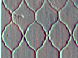
Image Sharpening
The so-called "unsharp mask" technique adds a fraction of the difference between a blurred version of the image and the original back to an image in order to further enhance the places that change most when blurred (i.e., image details).
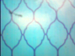
|

|
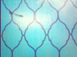
|
| Original Image | Blurred Image | Sharpened Image |
The kernel for the unsharp mask is a combination of the two steps, and may be written as
| 0 | –α | 0 |
| –α | (4α) + 1 | –α |
| 0 | –α | 0 |
where α is a sharpening factor (of your choice). You should note that the kernel is a combination of the 3×3 identity and a blurring kernel very similar to the Gaussian given above.
Oriented edge detectors
The Prewitt derivative operators (given above) identify strong brightness changes along a particular direction. Note that unlike the blurring kernels, these kernels sum to zero, so that when there is no change in an image the response is zero.
|
|
|

|
| Original Image | Horizontal Derivative KHoriz (Vertical Edges) |
Vertical Derivative KVert (Horizontal Edges) |
Because the filter responses may be positive or negative, centered
around zero, we must add a bias to place the results back into a
visible range. With the unsigned
char ranging from 0–255, using a bias of 128 will
center the responses so that zero appears gray, strong "positive"
edges appear brighter white, and strong "negative" edges appear
darker black.
Spot detection
The so-called Laplacian operator is the second derivative of a 2D Gaussian. Whereas the Gaussian looks like a bell when viewed as a 2D curve, the Laplacian has the shape of an inverted sombrero. Thus, it responds most strongly to a bright band surrounding a dark center. (It also responds less strongly to any edge.)
| 0.25 | 0.50 | 0.25 |
| 0.50 | –3.00 | 0.50 |
| 0.25 | 0.50 | 0.25 |
|
|
| Original Image | Laplacian |
As a differential operator whose kernel also sums to zero, a bias of 128 will aid in visualization.
Grading
In addition to the general grading guidelines for evaluation, the assignment is worth 30 points.
-
Comments on Program Format, Comments, Readability, etc.
(Points not given, but points can be deducted.) - [3 points] Function
trimoperates correctly - [11 points] Function
multiplyAdd- [7 points] Operates correctly for multiple kernel sizes, various locations, and bias terms
- [4 points] Verifies preconditions with assertions at invalid locations
- [6 points] Function
convolutionoperates correctly - [10 points] Function
main- [3 points] Loads original(s), displays and saves result images
- [5 points] Applies five distinct filters to image(s)
- [2 points] Describes non-example filter and intended effect
A five point penalty will apply to any submission that includes personally identifying information anywhere other than the references/honesty file.
